Integrating Satellite and Ground Measurements for Predicting Locations of Extreme Urban Heat


1
School of Urban Studies & Planning, Portland State University, Portland, OR 97201, USA
2
Science Museum of Virginia, Richmond, VA 23220, USA
*
Author to whom correspondence should be addressed.
Climate 2019, 7(1), 5; https://doi.org/10.3390/cli7010005
Submission received: 1 December 2018
/
Revised: 17 December 2018
/
Accepted: 22 December 2018
/
Published: 3 January 2019
(This article belongs to the Special Issue Climate Change, Heat Waves, and Human Health)
Abstract
:The emergence of urban heat as a climate-induced health stressor is receiving increasing attention among researchers, practitioners, and climate educators. However, the measurement of urban heat poses several challenges with current methods leveraging either ground based, in situ observations, or satellite-derived surface temperatures estimated from land use emissivity. While both techniques contain inherent advantages and biases to predicting temperatures, their integration may offer an opportunity to improve the spatial resolution and global application of urban heat measurements. Using a combination of ground-based measurements, machine learning techniques, and spatial analysis, we addressed three research questions: (1) How much do ambient temperatures vary across time and space in a metropolitan region? (2) To what extent can the integration of ground-based measurements and satellite imagery help to predict temperatures? (3) What landscape features consistently amplify and temper heat? We applied our analysis to the cities of Baltimore, Maryland, and Richmond, Virginia, and the District of Columbia using geocomputational machine learning processes on data collected on days when maximum air temperatures were above the 90th percentile of historic averages. Our results suggest that the urban microclimate was highly variable across all of the cities—with differences of up to 10 °C between coolest and warmest locations at the same time—and that these air temperatures were primarily dependent on underlying landscape features. Additionally, we found that integrating satellite data with ground-based measures provided highly accurate and precise descriptions of temperatures in all three study regions. These results suggest that accurately identifying areas of extreme urban heat hazards for any region is possible through integrating ground-based temperature and satellite data.
1. Introduction
Projections of global climate change under a high carbon emissions scenario [1] suggest that much of the world’s population will eventually endure an average annual surface temperature warming of 2 °C relative to the preindustrial period with significant amplification and lengthening of extreme heat waves. The impacts of high temperatures and increasing rate of heat waves affect many elements of urban infrastructure, including transport networks, power, potable water supply, food distribution networks, waste management facilities, and telecommunication networks. Urban heat poses an additional threat to human life, since it is the leading cause of weather-related fatalities and a major contributor to summertime morbidity and has specific impacts on those communities that are more vulnerable, such as those with pre-existing health conditions (e.g., chronic obstructive pulmonary disease, asthma, cardiovascular disease, etc.), limited access to resources, and the elderly. Excess heat limits the human body’s ability to regulate its internal temperature, which can result in increased cases of heat cramps, heat exhaustion, and heatstroke and may exacerbate other nervous system, respiratory, cardiovascular, genitourinary, and diabetes-related conditions [2].
While air conditioning provides relief from intense heat, the resulting increased energy use can place pressure on electricity infrastructure and raise the cost of electricity production [3,4]. Furthermore, higher electricity prices for low-income households can lead to energy poverty, reducing the capacity to live with proper environmental protection and raising the risk of excess mortality in both the summertime and wintertime [4]. As these conditions worsen with the rising frequency, duration, and intensity of extreme heat events, the need for methods to understand and adequately address the associated disparate impacts becomes essential.
Current approaches to describing the spatial distribution of urban heat can be characterized into two categories: ground-based measurements of ambient air temperature and satellite-derived land surface temperatures. Common methods of intra-urban heat analysis use thermal infrared (TIR) satellite data [5,6,7,8]. However, these methods do not present human-experienced ground-level temperature predictions due to the low resolution of satellite-based TIR band. Thus, it is inappropriate to use TIR-capable platforms such as Landsat or Advanced Spaceborne Thermal Emission and Reflection Radiometer (ASTER) for urban heat island effect (UHI) analyses in which human comfort and/or health are concerned [6]. The alternative approach is to collect ground-based measurements (“traverses”) and create models of observed temperatures across urban areas. This collection method has been used successfully both recently and before the existence of satellite-based TIR data [9,10,11,12,13,14,15]. Although the exact techniques vary, the overall methodology persists throughout the traverse-based literature: the use of moving temperature measurement devices throughout an urban environment to assess the changes in temperature, based on land use/land cover (LULC) configuration.
Within the traverse-based UHI literature, there has been a trend toward using spatial interpolation techniques to estimate the temperature in areas not visited by the mobile traverse [16]. We argue that an interpolation-based technique for traverse-based UHI is inadequate. Though some interpolation techniques include advanced features such as decay functions (Inverse Distance Weighting) and directionality (Kriging), they require spatial uniformity of observations in order to accurately estimate values for unobserved locations [17]. For a traverse-based temperature observation technique, no such uniform distributions of observation points have been observed in the literature at a city-wide scale.
In lieu of interpolating our observed temperature data, we employed a satellite pixel-based modeling approach similar to that of Land Use Regression for the creation of a continuous surface of predicted temperatures across our study areas. This method (described in detail in Section 3) used continuous raster-based LULC descriptors in combination with our temperature observations to build a model, which in turn was reapplied to our LULC descriptors to create a continuous surface of predicted temperatures for an entire urban area. Besides overcoming the errors and assumptions associated with spatial interpolation schemes, we noted that a major benefit of the model-based approach taken here was the ability to assess model diagnostics for strength of fit to observations (i.e., variance explained, expected error).
Using a combination of ground-based measurements, machine learning techniques, and spatial analysis, we addressed three research questions: (1) How much do ambient temperatures vary across time and space in a metropolitan region? (2) To what extent can the integration of ground-based measurements and satellite imagery help to predict temperatures? (3) What landscape features consistently amplify heat? We applied our analysis to the cities of Baltimore, Maryland (MD), and Richmond, Virginia (VA), and the District of Columbia (D.C.) using ground-based temperature data collected on days when air temperatures were well above the 90th percentile of historic averages.
2. Materials and Methods
2.1. Study Area
Our heat assessments took place in three mid-Atlantic cities in the USA: Richmond, VA, Baltimore, MD, and D.C. The city of Richmond, VA is located at approximately 37.5° North, 77.4° West, on the Falls of the James River just west of the Chesapeake Bay. Richmond covers approximately 162 km2, with a population of nearly 223,000 as of 2016 [18]. Over the past 30 years, summer temperatures in the Richmond area have average monthly highs of 29.2 °C, 31.2 °C, and 30.3 °C for June, July, and August, respectively, and on average the city experiences approximately 14 days above 35 °C annually. D.C. is located at approximately 38.9° North, 77.0° West, at the confluence of the Anacostia and Potomac rivers. D.C. covers approximately 177 km2, with a population of around 694,000 as of 2017 [18]. Summer temperatures in the D.C. area have average monthly highs of 29.0 °C, 31.3 °C, and 30.3 °C for June, July, and August, respectively, and on average D.C. experiences approximately 11 days above 35 °C annually. Baltimore, MD is located at approximately 39.3° North, 76.6° West, at the mouth of the Patapsco River west of Chesapeake Bay. Baltimore covers approximately 239 km2, with a population of around 615,000 as of 2016 [18]. Summer temperatures in the Baltimore region have average monthly highs of 28.3 °C, 30.7 °C, and 29.5 °C for June, July, and August, respectively, and on average Baltimore experiences approximately nine days above 35 °C annually.
2.2. Temperature Collection and Data
Data on temperatures were collected through vehicular traverses across the study area(s). This method uses vehicle-mounted temperature sensors along with a global positioning system (GPS), and has been used successfully in the past for UHI assessments [9,10,11,12,13,14,15,19,20]. Temperatures were collected at a one-second interval using a type “T” thermocouple and data logger. In order to track positionality of the recorded temperatures, we recorded latitudes and longitudes at a one-second interval using GPS devices. We divided individual study areas into sub-areas of varying sizes in which drivers had the ability to access a wide range of unique land uses/land covers (LULCs) within a one hour driving period. This maximization of traversing unique LULCs is important for subsequent modeling and analysis, as we wish to train our models on as many configurations of LULCs as exist in our study area. The focus on one-hour traverses aimed to capture a ‘snapshot’ of temperatures through the city, while allowing enough time for drivers to cover their assigned sub-areas. One-hour collection windows have proven to be adequate in previous analyses [9,12]. Statistics on the traverse-based data collection are found in Table 1.
Temperature observations collected during these campaigns were not conducted entirely by the authors but rather by a group of volunteers in each of the cities. Before each campaign was initiated, systematic community outreach to potential program partners was undertaken for each city through identifying and contacting “boundary organizations” whose mission and/or community-level work aligns with resilience building to climate change. This practice (loosely considered here as a form of collective leadership) enabled each of the organizations to then form collective and shared goals for the urban heat island data, while also allowing them reach out to their social and professional networks to gather sufficient volunteer interest to build the collection teams (usually one to two people per vehicle, though sometimes as many as four per vehicle in Richmond, VA). These volunteers, owing to their extensive backgrounds of working within the environmental, equity, and/or civic engagement landscape of their cities, were able to then offer each campaign a form of indigenous knowledge and experience of each city’s unique LULCs that the authors could never independently integrate before undertaking the projects.
After assembling this network of campaign volunteers and organizations in each city, a two-hour campaign orientation session on either the evening before or the day of temperature observation traverses was conducted. These orientation sessions introduced the volunteer teams to the physical phenomenon of urban heat islands, outlined several case studies of previous successful campaigns in other cities and their outcomes, and gave detailed explanations of and hands-on experiences with the campaign technology, as well as shared and collective construction of traverse routes through areas of interest. The volunteer teams then completed the traverses independent of each other and returned the temperatures sensors and GPS unit to the analysis team.
2.3. Spectral Data
In order to model observed temperatures based on LULCs, we used spectral data from the Sentinel-2 satellite constellation, provided by the European Space Agency. Sentinel-2 provides 13 separate bands, which provided information between 433–2280 nm on the electromagnetic spectrum (Table 2); [21]). The satellite had a temporal resolution of approximately 5 days and spatial resolutions of 10 m2 and 20 m2 for visible light and infrared, respectively. In addition, Sentinel-2 provided three 60 m2 bands which were optimized for atmospheric interference detection (bands 1, 9, and 10)—these were not included in the analysis due to their limited relationship to LULC [22]. Notably, Sentinel-2 did not capture thermal information, such as the commonly-used Landsat or ASTER platforms [23]—in other words, all spectral information in our analysis was based purely off of the surface reflectance of different LULCs within different bandwidths of the visible/infrared spectrum.
Often, analyses using satellite imagery combine several bands to create an index that describe specific LULC attributes, and categorize them such as ‘impervious surface’ or ‘vegetation’ [22]. Our analysis abstracted this classification by one level and used the raw spectral bands themselves, which were used to calculate different indices and land covers. Within the Washington, D.C. and Baltimore, MD study areas we conducted a brief analysis between two common satellite imagery indices and the bands of Sentinel-2. The first index used was the Normalized Difference Vegetation Index (NDVI), an index with values scaled from −1 (less vegetation) to 1 (more vegetation) [24]. NDVI is common in remote sensing literature and is often used for vegetation detection and change analyses [25,26]. The second index tested was the Normalized Built-up Area Index (NBAI), an index which associates higher values to impervious surfaces (including buildings) and lower values to water, soil, and vegetation [27].
2.4. Modeling
2.4.1. Focal Buffers
There are both direct and indirect ways the LULCs affect UHI in an area, and the configuration of LULCs within varying distances and clusters is important to understand—previous analyses have described a distance-decay effect in relation to LULCs and their impacts on temperatures at a given location [28,29]. This is, in effect. a realization of Tobler’s First Law of Geography, which states that “everything is related to everything else, but near things are more related than distant things” [30]. In order to reflect this principle in our analysis, we transformed each band in the analysis with a moving window average of varying spatial distances. This technique is not novel to our study and has played a central role in Land Use Regression literature [31,32,33,34]. The product of this analysis (henceforth referred to as a ‘focal buffer’) was a new raster dataset in which the pixel values represent the average value within a stated distance. For example, if the specified distance was 50 m and the specified band was “Band 2”, then the value of the output pixels from this analysis would reflect the average values in band 2 within 50 m. This analysis created focal buffers for each of the 10 analyzed bands (bands 2, 3, 4, 5, 6, 7, 8, 8A, 11, 12) at each of the distances defined in Voelkel and Shandas (2017) (e.g., 50 m, 100 m, 150 m, 200 m, 250 m, 300 m, 350 m, 400 m, 450 m, 500 m, 600 m, 700 m, 800 m, 900 m, 1000 m). The results of these analyses were 150 focal buffer rasters for each study location, which when combined provided us with a multi-distance, multi-spectral abstraction of LULC characteristics. The transformation of Sentinel-2 bands into these focal buffers allowed for a reduction in error associated with spatial autocorrelation as well as increasing model performance [34].
2.4.2. Data Compilation
An initial training data set was created by combining the observed temperatures and the focal buffers. This process involved the extraction of values from each of the 150 focal buffers at the locations of each of the observed temperature points. First, all 20 m2 band derivatives were resampled to 10 m2 in order to assess all variables on a pixel-by-pixel basis. In order to ameliorate some of the resolution discrepancies between the 1-s point collection, and 10 m2 (such as instances where multiple points would fall in the same pixel), bilinear interpolation was performed when assessing focal buffer values for each point. This practice recalculates values based on neighboring pixel values in a weighted manner dependent on the location of the temperature observation point within the pixel. The output of this analysis was a table with 151 variables (observed temperature and the values of each focal buffer) and a row for each observation. Overall, nine tables were created: for each study area, we built a separate table (and subsequent model) for each temperate collection period (morning, afternoon, and evening).
2.4.3. Random Forest Regression
To build a predictive model we selected Random Forest (RF) regression. RF is a nonparametric machine learning technique shown to produce highly-predictive classification and regression models in the field of remote sensing [12,22,31,34,35,36]. Although RF provides internal validation and randomization [37], we still performed cross validation due to its ability to detect over-fitting of RF models and present a more conservative estimate of predictive power [36,38]. To perform this cross validation, we randomly split each of our tables of temperatures and values (e.g., ‘Richmond-Morning’) into ‘training’ and ‘testing’ tables consisting of 70% of the data and 30% of the data, respectively. Each training table was used to build an RF model to predict the observed temperature values based on their measured LULC attributes. We use this training model to predict the remaining ‘test’ table—including the adjusted R2 and Root Mean Square Error, which are both measures of predictive capacity—to compare the observed versus predicted values. Once an appropriate model was acquired, it was combined with the 150 focal buffer rasters to predict a continuous surface of temperatures. This process works by assessing the focal buffer values for each pixel in the study area, feeding it through the RF model, and assigning the predicted temperature values to their corresponding geographically-located pixel.
3. Results
3.1. Urban Heat Island Modeling
Overall, all nine models showed high predictive power (adjusted R2) and low RMSE values (Table 3). Across all models, we observed no less than 96.44% of the variation in observed temperatures explained by the focal buffers with an average R2 of 0.9818. In addition, the maximum observed RMSE was 0.1837 °C during the afternoon model in Baltimore, MD. The average RMSE was 0.1276 °C. As noted in previous studies, the afternoon models had a consistently lower performance and were likely attributed to more detailed descriptions of urban environments such as variations in humidity, building heights, and the effects therein on wind patterns and building density [12].
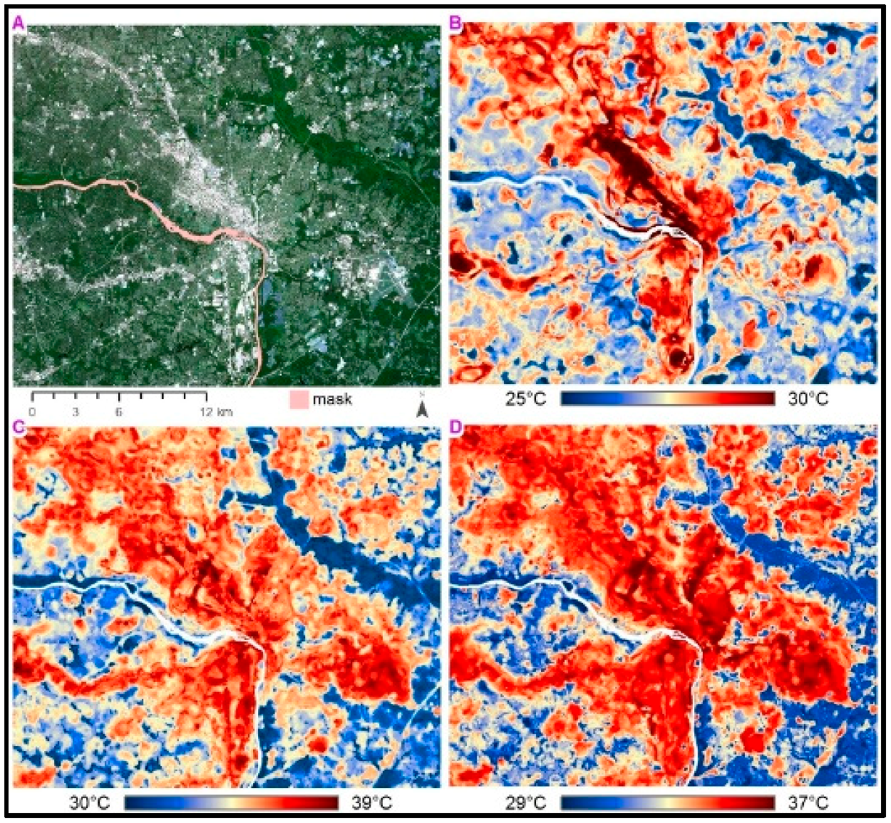
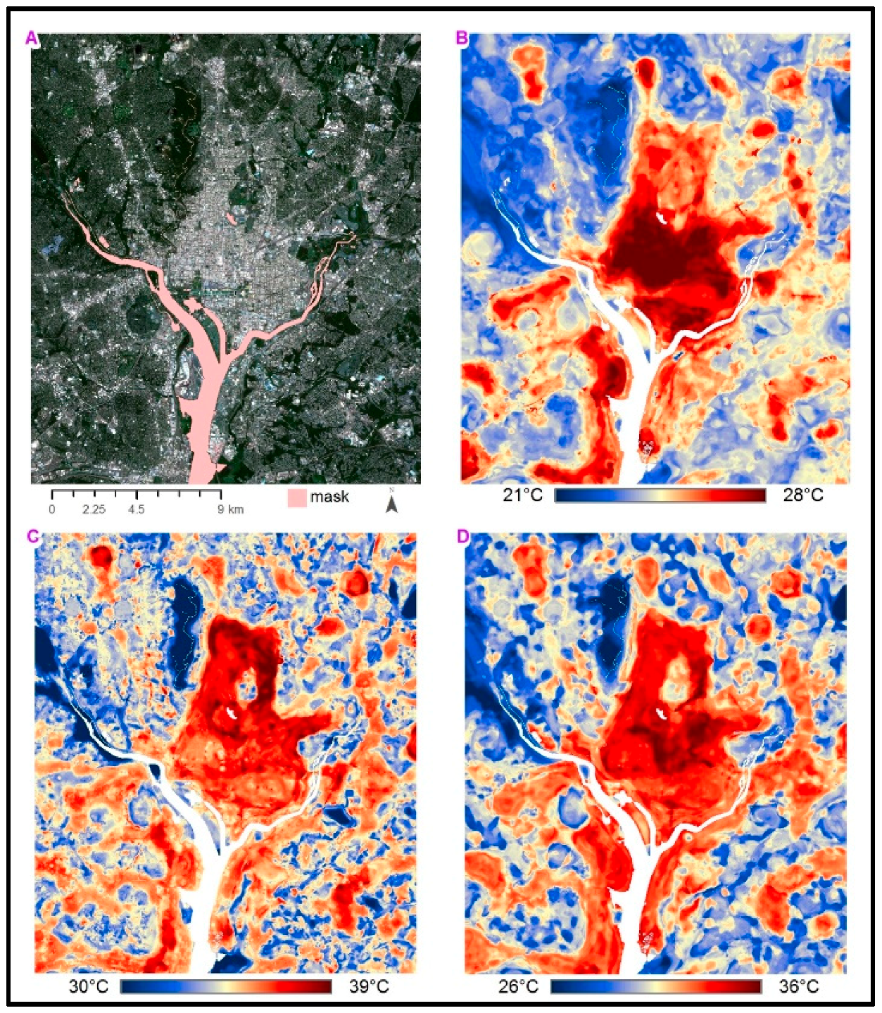
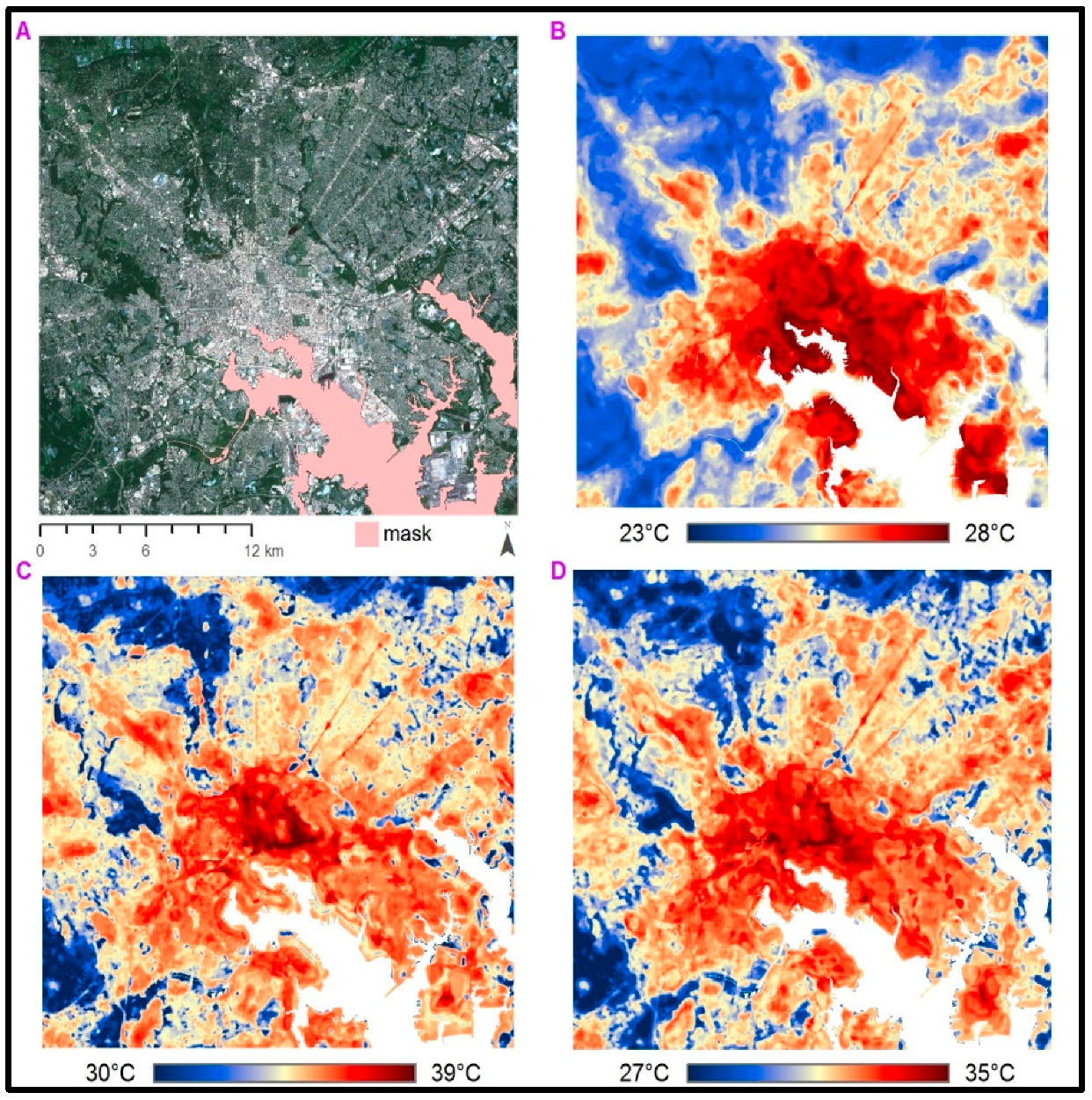
Across all three study areas, common patterns were observed: forested and otherwise vegetated areas are cooler than urbanized areas; lower-density urban areas are often cooler than high-density urban areas; morning high temperatures are always lower than afternoon and evening low temperatures; the greatest relative concentration of heat is in the morning; major arterial roadways are visible in all UHI surfaces, though they are often amplified in the evening (Figure 1, Figure 2 and Figure 3). High density, sparsely vegetated areas near major arterial roadways appear to consistently amplify heat within these metropolitan regions.
3.2. Land Cover/Band Correlations
Results from the correlation analysis between land classification-linked indices and raw Sentinel-2 bands indicate the strongest correlations between the Normalized Difference Vegetation Index (NDVI), which is a measure of total vegetation, and Normalized Built-up Area Index (NBAI), which is a measure of built up area (e.g., roads, buildings, driveways, etc.). The NDVI had the highest correlations to band 8 (R = 0.89), band 2 (R = −0.32), and band 4 (R = −0.29), while the NBAI had strong correlations to band 4 (R = 0.74), band 2 (R = 0.70), and band 3 (R = 0.69) (Table 4). The evaluation of each Sentinel band with the two remotely sensed indices suggests that the raw information contained in the Sentinel-2 bands reflect abstract descriptions of LULC.
4. Discussion
This study aimed to address three research questions relevant to: (1) the variation of ambient temperatures; (2) predicting temperatures using ground and satellite data; and (3) the role of landscape features in amplifying temperatures. The results indicate that in all of our study regions, the temperatures vary by over 10 °C, and that those patterns were largely due to specific land cover patterns, including the presence of dense buildings (hottest) and parks/open space (coolest), which is consistent with other UHI studies using similar traverse-based methods [10,11,12,13,14,15]. The study went further to illustrate that specific satellite bands can help to inform predictions about the distribution of urban heat. In fact, within the model diagnostics, we observed that the application of a machine learning technique (RF) created high performing models with excellent predictive power, and low variance in error (RMSE).
4.1. Land Cover/Band Correlations
The finding that NDVI and NBAI are highly correlated with certain Sentinel-2 bands is neither novel nor groundbreaking; however, it is illustrative for our study. Commonly, studies use such indices for the classification of specific LULCs (e.g., ‘impervious surface’, ‘vegetation’) and proceed to perform analyses. By including all pertinent (i.e., removing the 60 m bands) Sentinel-2 bands in our study, we are providing the RF machine learning model with the information often used to classify LULC [39,40,41], and also the information necessary to continue one step further and model temperatures. In summary, the results suggest that RF offers a direct means for accurately classify LULCs from Sentinel-2 bands, and to predict ambient temperatures.
4.2. Implications for Understanding Extreme Heat in Mid-Atlantic Cities
Official air temperature maxima reported for our study areas (Richmond, Baltimore, and Washington DC’s National airports) on the dates of our heat island assessments were systematically lower by an average of 4.6 °C (>8 °F) than the maximum temperatures observed during our traverses (Table 1), and those modeled in our heat surfaces. Static, sensor-based studies of urban minimum air temperatures in the City of Baltimore [42] previously identified LULC as a significant predictor of temperature minimums, though it has a three limitations, which the present study addresses. First, while this and earlier studies confirmed a distribution of temperatures across urban areas, they often failed to correlate those differences to land use types such as tree canopy and distance from park areas. Second, the placement of stationary sensors may provide high temporal variability, though with a large physical extent like Baltimore, spatial extent to capture diversity LULC is essential for model validity. Finally, while an ordinary least square regression provides specific coefficients, the integration of RF is a significant advancement in the capacity for predicting temperatures, and hence, offers a means for actively addressing planning options. In addition, our modeled and observed minimum temperature range for Baltimore (Figure 3b) far exceeded that of previous studies, which provides further evidence for applying RF to produce highly predictive temperature surfaces as well as traverse observations. Ongoing work with other cities across the country will likely corroborate findings using sensor-based estimates of ambient urban temperatures.
The results suggest that some neighborhoods contain higher heat during an individual event, and may also have significantly longer heat seasons. Extreme heat warnings issued by the National Weather Service before and during heat waves may rely solely on temperatures from these official stations, thereby inadvertently underestimating the apparent health risk to communities that suffer higher urban heat. These temperature maps can help to prioritize action areas for engaging those neighborhoods that are consistently hotter than official temperature records. Additionally, long-term temperature measurement and monitoring can help to inform the timing of public health warnings about heat. Understanding how the built environments amplify or mitigate extreme heat within specific neighborhoods is critical to building resilience to future heat extremes.
Additionally, our findings highlight the clear need to better understand the interactions between areas containing extreme urban heat and socioeconomic factors that may describe the adaptive capacity of the community. Throughout the campaign, volunteers noted the relationship between lower income areas of each city and the lack of heat mitigating features, including trees, open space, and/or lighter coloring on surfaces. While an increasing body of literature is confirming these anecdotal claims, having precise and accurate predictions of urban heat within all urban areas will help to advance preventative measures for reducing far-reaching impacts from future heat events.
One promising direction is the use of public health records that can identify acute vulnerabilities to urban heat within the community, which offer means for identifying equitable policies and strategies that seek to alleviate the burden of extreme heat on vulnerable communities [42]. This may include focusing research attention on high-resolution, city-scale climate modeling where future redevelopment and land use change is incorporated alongside projected increases to air temperature, extreme precipitation, and other climate change impacts such as sea-level change and the intrusion of invasive species into urban areas. Future work will explore and show how boundary organizations and volunteers included in these heat assessment campaigns have since leveraged this study’s findings to advocate for, design, and implement resilience strategies in their respective cities.
5. Conclusions
Emerging tools can further help to apply urban heat assessments across the United States or globally. Climate Engine, an on-demand processor of satellite and climate data, provides an extensive set of variables for examination of climate impacts such as extreme heat, drought, and wildfire [43]. Climate Engine uses remote sensing data from platforms such as Landsat 4, 5, 7, and 8, and Moderate Resolution Imaging Spectroradiometer (MODIS) Terra to quickly assess, analyze, and visualize hazard and population information at various scales over large areas [43,44]. Moreover, remote sensing data may serve to inform decision-making frameworks, such as the National Oceanic and Atmospheric Administration’s (NOAA) Climate Resilience Toolkit. With enhanced informing of hazards and vulnerabilities, communities may be empowered through the Toolkit to better evaluate risks and costs associated with natural disasters such as extreme heat and develop appropriate mitigation and adaptation solutions [45]. Other efforts by civic leaders and organizations aim to coordinate resilience activities across cities and regions while engaging citizens to take action in their communities.
The novel framework described in the present study offers researchers the ability to measure and understand community exposure to extreme heat. Using volunteer-based, community science-led urban heat assessments provides a direct means for low-cost, and highly predicative descriptions of temperature. Our in situ observations and model surfaces for three Mid-Atlantic metropolitan regions point to substantial and land-use specific variation in ambient temperatures across time and space, on the order of ~10 °C for the same time period and up to ~18 °C throughout the diurnal cycle (Table 2), addressing research question (1) and, in part, research question (2). Through combining both satellite-derived and in situ data, our heat island model surfaces are shown to be highly predictive within several dense urban environments spanning the Mid-Atlantic region, an area of the USA that is acutely impacted by increasing extreme heat waves [1]. We identified extreme disparity in air temperature maximums within our study areas that is dominantly controlled and amplified by land use features such as dense, sparsely vegetated urban cores and major arterial roadways, regardless of latitude and areal extent. As a result, our study underscores the need for assessments for current climate vulnerabilities, and for potential future climate change exacerbation. We offered the maps as rhetorical tools for public discourse, and as examples of finding mechanisms to develop city-scale resilience plans, one neighborhood at a time.
With enhanced information about the scale of worsening hazards and vulnerabilities, communities may be empowered with increasingly precise and accurate heat data to better evaluate exposure, sensitivity, and vulnerability to worsening natural disasters like extreme heat. Additionally, the method described here highlights how civic leaders, resilience boundary organizations, and cultural institutions (such as science centers and museums) can coordinate climate resilience-building activities across cities and regions while engaging community members to take climate action within their neighborhoods. As climate change continues to increase the duration, intensity, and frequency of extreme heat waves, concomitantly with further expansion and densification of urban areas, collaborative informational field campaigns can provide actionable data for decision makers for any region.
Author Contributions
V.S. conceived of and collected the data for the study and contributed to the writing of the full manuscript. J.V. participated in the collection of field data from Richmond, V.A., performed the analysis, and wrote parts of the methods and results sections. J.W. contributed to the collection of relevant materials and field data from Baltimore and Washington DC field locations, formatting, and some writing of the manuscript. J.H. contributed to the collection of data from all the study locations and writing of the manuscript.
Funding
This research was funded by the National Oceanic and Atmospheric Administration’s Community, Education and Engagement Division, the National Oceanic and Atmospheric Administration’s Office of Education Environmental Literacy Program (Award Number NA15SEC0080009), the Virginia Academy of Science, and the National Science Foundation’s Sustainable Research Network Grant (No. 1444755).
Acknowledgments
This research was made possible with support from the Institute of Sustainable Solutions at Portland State University, and the James F. & Marion L. Miller Foundation. The authors also acknowledge the teams of volunteers from each of the study areas who carefully and dutifully completed their traverses and contributed to the positive outcomes and success of these projects. The authors further acknowledge GroundworkRVA in Richmond, the National Aquarium in Baltimore, Science Museum of Virginia, and the Department of Energy and Environment in Washington, D.C. for opening up their facilities for the volunteer training orientation sessions.
Conflicts of Interest
The authors declare no conflict of interest. The funders had no role in the design of the study; in the collection, analyses, or interpretation of data; in the writing of the manuscript, or in the decision to publish the results.
References
- Riahi, K.; Rao, S.; Krey, V.; Cho, C.; Chirkov, V.; Fischer, G.; Kindermann, G.; Nakicenovic, N.; Rafaj, P. RCP 8.5—A scenario of comparatively high greenhouse gas emissions. Clim. Chang. 2011, 109, 33. [Google Scholar] [CrossRef]
- Uejio, C.K.; Wilhelmi, O.V.; Golden, J.S.; Mills, D.M.; Gulino, S.P.; Samenow, J.P. Intra-urban societal vulnerability to extreme heat: The role of heat exposure and the built environment, socioeconomics, and neighborhood stability. Health Place 2011, 17, 498–507. [Google Scholar] [CrossRef] [PubMed]
- Hatvani-Kovacs, G.; Belusko, M.; Pockett, J.; Boland, J. Assessment of Heatwave Impacts. Procedia Eng. 2016, 169, 316–323. [Google Scholar] [CrossRef]
- Santamouris, M.; Kolokotsa, D. On the impact of urban overheating and extreme climatic conditions on housing, energy, comfort and environmental quality of vulnerable population in Europe. Energy Build. 2015, 98, 125–133. [Google Scholar] [CrossRef]
- Klok, L.; Zwart, S.; Verhagen, H.; Mauri, E. The surface heat island of Rotterdam and its relationship with urban surface characteristics. Resour. Conserv. Recycl. 2012, 64, 23–29. [Google Scholar] [CrossRef]
- Sobrino, J.A.; Oltra-Carrió, R.; Sòria, G.; Bianchi, R.; Paganini, M. Impact of spatial resolution and satellite overpass time on evaluation of the surface urban heat island effects. Remote Sens. Environ. 2012, 117, 50–56. [Google Scholar] [CrossRef]
- Stathopoulou, M.; Cartalis, C. Daytime urban heat islands from Landsat ETM+ and Corine land cover data: An application to major cities in Greece. Sol. Energy 2007, 81, 358–368. [Google Scholar] [CrossRef]
- Zhang, Y.; Murray, A.T.; Turner, B.L. Optimizing green space locations to reduce daytime and nighttime urban heat island effects in Phoenix, Arizona. Landsc. Urban Plan. 2017, 165, 162–171. [Google Scholar] [CrossRef] [Green Version]
- Sailor, D.J.; Smith, M.; Hart, M. Climate change implications for wind power resources in the Northwest United States. Renew. Energy 2008, 33, 2393–2406. [Google Scholar] [CrossRef]
- Makido, Y.; Shandas, V.; Ferwati, S.; Sailor, D. Daytime Variation of Urban Heat Islands: The Case Study of Doha, Qatar. Climate 2016, 4, 32. [Google Scholar] [CrossRef]
- Saaroni, H.; Ben-Dor, E.; Bitan, A.; Potchter, O. Spatial distribution and microscale characteristics of the urban heat island in Tel-Aviv, Israel. Landsc. Urban Plan. 2000, 48, 1–18. [Google Scholar] [CrossRef]
- Voelkel, J.; Shandas, V. Towards Systematic Prediction of Urban Heat Islands: Grounding Measurements, Assessing Modeling Techniques. Climate 2017, 5, 41. [Google Scholar] [CrossRef]
- Wong, N.H.; Yu, C. Study of green areas and urban heat island in a tropical city. Habitat Int. 2005, 29, 547–558. [Google Scholar] [CrossRef]
- Yamashita, S.; Sekine, K.; Shoda, M.; Yamashita, K.; Hara, Y. On relationships between heat island and sky view factor in the cities of Tama River basin, Japan. Atmos. Environ. 1967 1986, 20, 681–686. [Google Scholar] [CrossRef]
- Yokobori, T.; Ohta, S. Effect of land cover on air temperatures involved in the development of an intra-urban heat island. Clim. Res. 2009, 39, 61–73. [Google Scholar] [CrossRef] [Green Version]
- Kardinal Jusuf, S.; Wong, N.H.; Hagen, E.; Anggoro, R.; Hong, Y. The influence of land use on the urban heat island in Singapore. Habitat Int. 2007, 31, 232–242. [Google Scholar] [CrossRef]
- Jeffrey, S.J.; Carter, J.O.; Moodie, K.B.; Beswick, A.R. Using spatial interpolation to construct a comprehensive archive of Australian climate data. Environ. Model. Softw. 2001, 16, 309–330. [Google Scholar] [CrossRef]
- United States Census Bureau American Fact Finder. Available online: https://factfinder.census.gov/ (accessed on 2 January 2019).
- Chandler, T.J. Temperature and Humidity Traverses Across London. Weather 1962, 17, 235–242. [Google Scholar] [CrossRef]
- Kotharkar, R.; Surawar, M. Land Use, Land Cover, and Population Density Impact on the Formation of Canopy Urban Heat Islands through Traverse Survey in the Nagpur Urban Area, India. J. Urban Plan. Dev. 2016, 142, 04015003. [Google Scholar] [CrossRef]
- GMES Sentinel-2 Mission Requirements Document. Available online: https://earth.esa.int/pub/ESA_DOC/GMES_Sentinel2_MRD_issue_2.0_update.pdf (accessed on 2 January 2019).
- Sonobe, R.; Yamaya, Y.; Tani, H.; Wang, X.; Kobayashi, N.; Mochizuki, K. Evaluating metrics derived from Landsat 8 OLI imagery to map crop cover. Geocarto Int. 2018. [Google Scholar] [CrossRef]
- Ramachandran, B.; Justice, C.O.; Abrams, M.J. Land Remote Sensing and Global Environmental Change: NASA’s Earth Observing System and the Science of ASTER and MODIS; Springer Science & Business Media: Berlin, Germany, 2010; ISBN 978-1-4419-6749-7. [Google Scholar]
- Monitoring the Vernal Advancement and Retrogradation (Green Wave Effect) of Natural Vegetation. Available online: https://ntrs.nasa.gov/archive/nasa/casi.ntrs.nasa.gov/19750020419.pdf (accessed on 2 January 2019).
- Gandhi, G.M.; Parthiban, S.; Thummalu, N.; Christy, A. Ndvi: Vegetation Change Detection Using Remote Sensing and Gis—A Case Study of Vellore District. Procedia Comput. Sci. 2015, 57, 1199–1210. [Google Scholar] [CrossRef]
- Running, S.W.; Loveland, T.R.; Pierce, L.L.; Nemani, R.R.; Hunt, E.R. A remote sensing based vegetation classification logic for global land cover analysis. Remote Sens. Environ. 1995, 51, 39–48. [Google Scholar] [CrossRef]
- Valdiviezo-N, J.C.; Téllez-Quiñones, A.; Salazar-Garibay, A.; López-Caloca, A.A. Built-up index methods and their applications for urban extraction from Sentinel 2A satellite data: Discussion. JOSA A 2018, 35, 35–44. [Google Scholar] [CrossRef] [PubMed]
- Shashua-Bar, L.; Hoffman, M.E. Vegetation as a climatic component in the design of an urban street: An empirical model for predicting the cooling effect of urban green areas with trees. Energy Build. 2000, 31, 221–235. [Google Scholar] [CrossRef]
- Voelkel, J.; Shandas, V.; Haggerty, B. Developing High-Resolution Descriptions of Urban Heat Islands: A Public Health Imperative. Prev. Chronic. Dis. 2016, 13, E129. [Google Scholar] [CrossRef] [PubMed]
- Tobler, W.R. A Computer Movie Simulating Urban Growth in the Detroit Region. Econ. Geogr. 1970, 46, 234–240. [Google Scholar] [CrossRef]
- Clougherty, J.E.; Kheirbek, I.; Eisl, H.M.; Ross, Z.; Pezeshki, G.; Gorczynski, J.E.; Johnson, S.; Markowitz, S.; Kass, D.; Matte, T. Intra-urban spatial variability in wintertime street-level concentrations of multiple combustion-related air pollutants: The New York City Community Air Survey (NYCCAS). J. Expo. Sci. Environ. Epidemiol. 2013, 23, 232–240. [Google Scholar] [CrossRef]
- Henderson, S.B.; Beckerman, B.; Jerrett, M.; Brauer, M. Application of Land Use Regression to Estimate Long-Term Concentrations of Traffic-Related Nitrogen Oxides and Fine Particulate Matter. Environ. Sci. Technol. 2007, 41, 2422–2428. [Google Scholar] [CrossRef]
- Rao, M.; George, L.A.; Rosenstiel, T.N.; Shandas, V.; Dinno, A. Assessing the relationship among urban trees, nitrogen dioxide, and respiratory health. Environ. Pollut. Barking Essex 1987 2014, 194, 96–104. [Google Scholar] [CrossRef]
- Rodriguez-Galiano, V.F.; Chica-Olmo, M.; Abarca-Hernandez, F.; Atkinson, P.M.; Jeganathan, C. Random Forest classification of Mediterranean land cover using multi-seasonal imagery and multi-seasonal texture. Remote Sens. Environ. 2012, 121, 93–107. [Google Scholar] [CrossRef]
- Ghimire, B.; Rogan, J.; Miller, J. Contextual land-cover classification: Incorporating spatial dependence in land-cover classification models using random forests and the Getis statistic. Remote Sens. Lett. 2010, 1, 45–54. [Google Scholar] [CrossRef]
- Oliveira, S.; Oehler, F.; San-Miguel-Ayanz, J.; Camia, A.; Pereira, J.M. c. Modeling spatial patterns of fire occurrence in Mediterranean Europe using Multiple Regression and Random Forest. For. Ecol. Manag. 2012, 275, 117–129. [Google Scholar] [CrossRef]
- Hastie, T. The Elements of Statistical Learning: Data Mining, Inference, and Prediction, 2nd ed.; Springer Series in Statistics; Springer: New York, NY, USA, 2009; ISBN 978-0-387-84857-0. [Google Scholar]
- Dormann, C.F.; Elith, J.; Bacher, S.; Buchmann, C.; Carl, G.; Carré, G.; Marquéz, J.R.G.; Gruber, B.; Lafourcade, B.; Leitão, P.J.; et al. Collinearity: A review of methods to deal with it and a simulation study evaluating their performance. Ecography 2013, 36, 27–46. [Google Scholar] [CrossRef]
- Huang, G.; Zhou, W.; Cadenasso, M.L. Is everyone hot in the city? Spatial pattern of land surface temperatures, land cover and neighborhood socioeconomic characteristics in Baltimore, MD. J. Environ. Manag. 2011, 92, 1753–1759. [Google Scholar] [CrossRef] [PubMed]
- Mallick, J.; Rahman, A.; Singh, C.K. Modeling urban heat islands in heterogeneous land surface and its correlation with impervious surface area by using night-time ASTER satellite data in highly urbanizing city, Delhi-India. Adv. Space Res. 2013, 52, 639–655. [Google Scholar] [CrossRef]
- Rodriguez-Galiano, V.F.; Ghimire, B.; Rogan, J.; Chica-Olmo, M.; Rigol-Sanchez, J.P. An assessment of the effectiveness of a random forest classifier for land-cover classification. ISPRS J. Photogramm. Remote Sens. 2012, 67, 93–104. [Google Scholar] [CrossRef]
- Scott, A.A.; Zaitchik, B.; Waugh, D.W.; O’Meara, K. Intraurban Temperature Variability in Baltimore. J. Appl. Meteorol. Climatol. 2016, 56, 159–171. [Google Scholar] [CrossRef]
- Kerle, N. Remote sensing of natural hazards and disasters. Encycl. Nat. Hazards 2013, 837–847. [Google Scholar] [CrossRef]
- Huntington, J.L.; Hegewisch, K.C.; Daudert, B.; Morton, C.G.; Abatzoglou, J.T.; McEvoy, D.J.; Erickson, T. Climate Engine: Cloud Computing and Visualization of Climate and Remote Sensing Data for Advanced Natural Resource Monitoring and Process Understanding. Bull. Am. Meteorol. Soc. 2017, 98, 2397–2410. [Google Scholar] [CrossRef]
- National Oceanic and Atmospheric Administration Climate Program Office U.S. Climate Resilience Toolkit. Available online: https://toolkit.climate.gov/content/us-climate-resilience-toolkit (accessed on 29 November 2018).
Figure 1.
Richmond, VA (A) aerial imagery with major waterbodies masked; (B) morning urban heat island (UHI); (C) afternoon UHI; (D) evening UHI.
Figure 1.
Richmond, VA (A) aerial imagery with major waterbodies masked; (B) morning urban heat island (UHI); (C) afternoon UHI; (D) evening UHI.

Figure 2.
Washington, D.C. (A) aerial imagery with major waterbodies masked; (B) morning UHI; (C) afternoon UHI; (D) evening UHI.
Figure 2.
Washington, D.C. (A) aerial imagery with major waterbodies masked; (B) morning UHI; (C) afternoon UHI; (D) evening UHI.

Figure 3.
Baltimore, MD (A) aerial imagery with major waterbodies masked; (B) morning UHI; (C) afternoon UHI; (D) evening UHI.
Figure 3.
Baltimore, MD (A) aerial imagery with major waterbodies masked; (B) morning UHI; (C) afternoon UHI; (D) evening UHI.


Table 1.
Overview of temperature collections and data.
| Study Area | Area Covered (km2) | Date | n | Number of Drivers | Observed Temperatures (°C) | |||
|---|---|---|---|---|---|---|---|---|
| Min. | Mean | Med. | Max. | |||||
| Richmond, VA | 851 | 13 July 2017 | 103,971 | 12 (9 cars, 3 bicycles) | 24.8 | 31.8 | 33.6 | 39.5 |
| Washington, D.C. | 476 | 28 August 2018 | 74,048 | 9 cars | 20.5 | 30.5 | 32.0 | 39.5 |
| Baltimore, MD | 679 | 29 August 2018 | 79,306 | 9 cars | 22.4 | 30.8 | 31.8 | 40.3 |
Table 2.
Sentinel-2 bands.
| Band | Purpose | Wavelength (nm) | Spatial Resolution (m2) |
|---|---|---|---|
| 1 | Coastal aerosols | 443 | 60 |
| 2 | Blue | 490 | 10 |
| 3 | Green | 560 | 10 |
| 4 | Red | 665 | 10 |
| 5 | Vegetation red edge | 705 | 20 |
| 6 | Vegetation red edge | 740 | 20 |
| 7 | Vegetation red edge | 783 | 20 |
| 8 | NIR * | 842 | 10 |
| 8A | Narrow NIR | 865 | 20 |
| 9 | Water vapour | 940 | 60 |
| 10 | SWIR **/Cirrus | 1375 | 60 |
| 11 | SWIR | 1610 | 20 |
| 12 | SWIR | 2190 | 20 |
*: Near infrared.; **: Shortwave infrared.
Table 3.
Model Results.
| Study Area | Time | R2 | RMSE |
|---|---|---|---|
| Richmond, VA | Morning | 0.9795 | 0.0809 |
| Afternoon | 0.9644 | 0.1782 | |
| Evening | 0.9764 | 0.1304 | |
| Washington, D.C. | Morning | 0.9967 | 0.0650 |
| Afternoon | 0.9803 | 0.1737 | |
| Evening | 0.9928 | 0.1156 | |
| Baltimore, MD | Morning | 0.9923 | 0.0871 |
| Afternoon | 0.9685 | 0.1837 | |
| Evening | 0.9850 | 0.1334 |
Table 4.
Correlations between common land use-linked indices and raw Sentinel-2 bands.
| Sentinel-2 Band | Index | |
|---|---|---|
| NDVI | NBAI | |
| B2 | −0.3249 | 0.7011 |
| B3 | −0.2452 | 0.6884 |
| B4 | −0.2941 | 0.7378 |
| B5 | 0.0019 | −0.0002 |
| B6 | 0.0085 | −0.0003 |
| B7 | 0.0080 | −0.0004 |
| B8 | 0.8896 | −0.4800 |
| B8A | 0.0073 | −0.0004 |
| B11 | 0.0051 | −0.0008 |
| B12 | 0.0036 | −0.0006 |
© 2019 by the authors. Licensee MDPI, Basel, Switzerland. This article is an open access article distributed under the terms and conditions of the Creative Commons Attribution (CC BY) license (http://creativecommons.org/licenses/by/4.0/).
Share and Cite
MDPI and ACS Style
Shandas, V.; Voelkel, J.; Williams, J.; Hoffman, J. Integrating Satellite and Ground Measurements for Predicting Locations of Extreme Urban Heat. Climate 2019, 7, 5. https://doi.org/10.3390/cli7010005
AMA Style
Shandas V, Voelkel J, Williams J, Hoffman J. Integrating Satellite and Ground Measurements for Predicting Locations of Extreme Urban Heat. Climate. 2019; 7(1):5. https://doi.org/10.3390/cli7010005
Chicago/Turabian StyleShandas, Vivek, Jackson Voelkel, Joseph Williams, and Jeremy Hoffman. 2019. "Integrating Satellite and Ground Measurements for Predicting Locations of Extreme Urban Heat" Climate 7, no. 1: 5. https://doi.org/10.3390/cli7010005
Note that from the first issue of 2016, this journal uses article numbers instead of page numbers. See further details here.